S&P 500 Betting with Transformers
Overview
The task of this competition is to predict the stock market returns as represented by the excess returns of the S&P 500 while also managing volatility constraints. Your work will test the Efficient Market Hypothesis and challenge common tenets of personal finance. Furthere details about the competition can be found here.
Problem Statement
Wisdom from most personal finance experts would suggest that it's irresponsible to try and time the market. The Efficient Market Hypothesis (EMH) would agree: everything knowable is already priced in, so don't bother trying. But in the age of machine learning, is it irresponsible to not try and time the market? Is the EMH an extreme oversimplification at best and possibly just…false?
Predicting market returns challenges the assumptions of market efficiency. Your work could help reshape how investors and academics understand financial markets. Participants could uncover signals others overlook, develop innovative strategies, and contribute to a deeper understanding of market behavior—potentially rewriting a fundamental principle of modern finance. Most investors don't beat the S&P 500. That failure has been used for decades to prop up EMH: If even the professionals can't win, it must be impossible. This observation has long been cited as evidence for the Efficient Market Hypothesis the idea that prices already reflect all available information and no persistent edge is possible. This story is tidy, but reality is less so. Markets are noisy, messy, and full of behavioral quirks that don't vanish just because academic orthodoxy said they should. This competition asks to build a model that predicts excess returns and includes a betting strategy designed to outperform the S&P 500 while staying within a 120% volatility constraint.
Technical Approach
Model Procedure
My approach is to use a transformer encoder neural network model with an allocation head to give values between 0, representing no leverage entered into the market, and 2, representing 2x leverage in the market. This model first normalizes and embeds the input features into an embedding layer. It then applies positional encoding to provide the mechanism a sense of time ordering, which is then fed into the transformer encoder. More reading about the transformer encoder can be found here. The transformer outputs a context matrix \(Z\) with the same dimension as the input \(X_{input}\). Each row of Z represents a different lagged set of mixed features.
The final allocation head first flattens the context matrix \(Z\), creating a feature vector. A final neural network layer is applied to the feature vector using a sigmoid activation function, which outputs values between [0,1]. This is then scaled by 2 to get the allocations per day. Therefore model is trained on the actions it takes, not on its prediction of future returns. I use a custom loss function which is a modified negative sharpe ratio. The objective is to maximize the sharpe ratio by minimizing the negative sharpe loss.
Results & Impact
During training, 20 percent of the training set was used for validation. After training, the training sharpe ratio is 0.026 while the validation sharpe ratio is 1.85. This could be that the validation set is small, which allows the model to overachieve.
Training Dataset
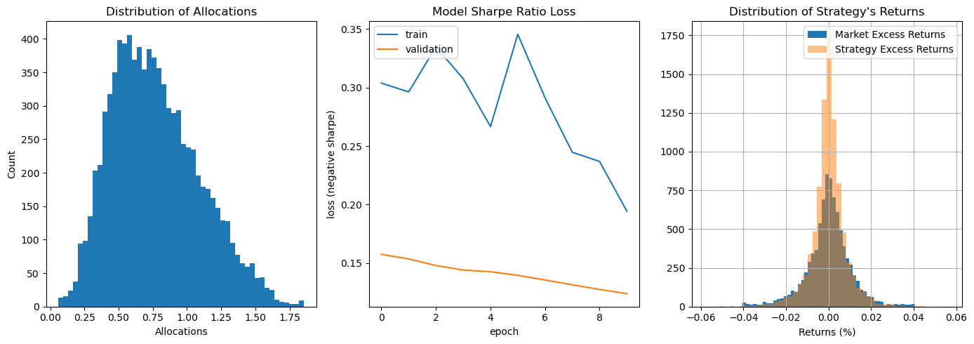
Figure 1: The distribution of allocations for the train dataset as well as the training and validation loss values.
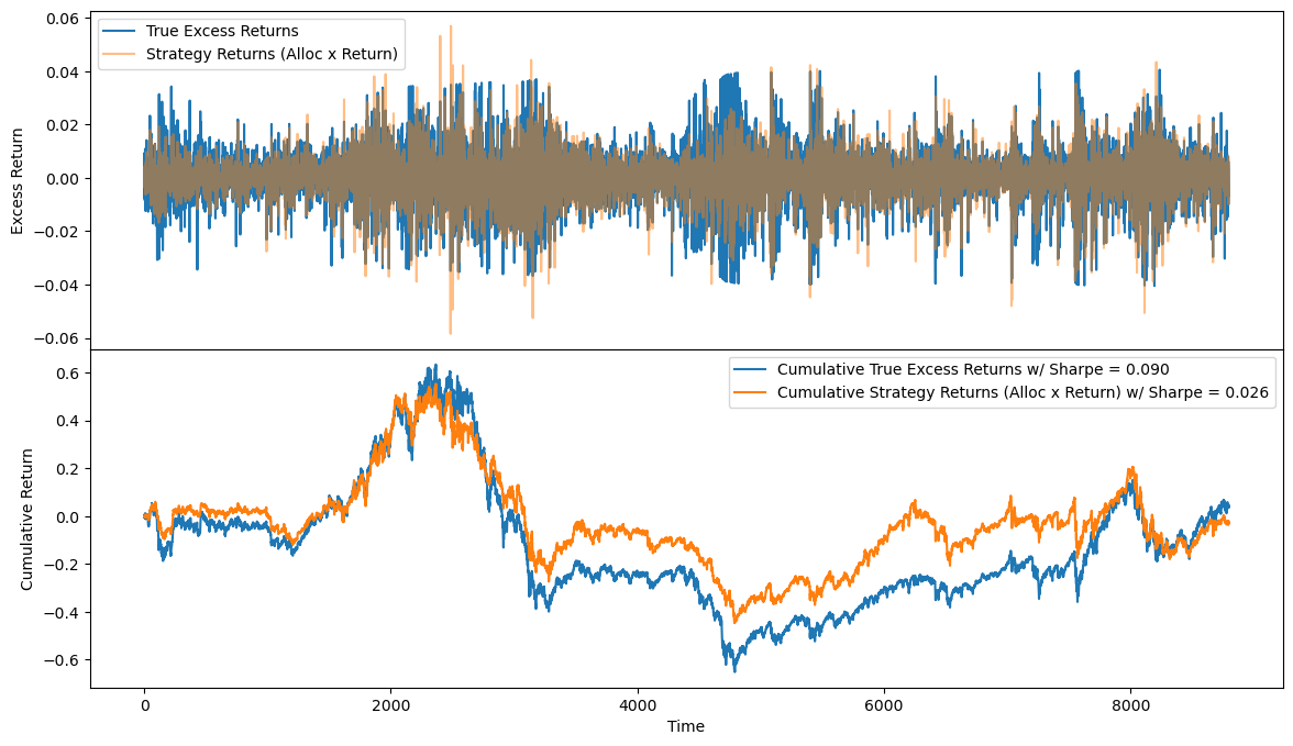
Figure 2: The order parameter that measures general synchronization among all the indexes over time.
I used the model to produce allocations for the entire training dataset. The resulting sharpe ratio was ~0.03, which is out-performed by the market (if each allocation was 1) with a sharpe of 0.09. The distribution of allocations, the training and validation loss plot, and the distribution of returns can be seen in Figure 1. The cumulative excess returns of both the model's strategy and the S&P 500 are shown in Figure 2.
Test Dataset
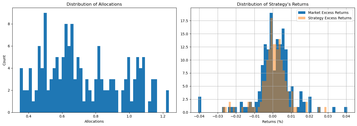
Figure 1: The distribution of allocations for the test dataset.
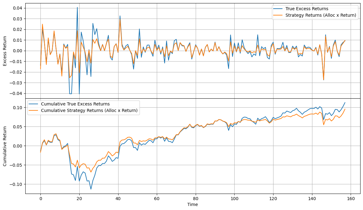
Figure 2: The resulting test returns for both the market and the model.
The model was then applied on the test dataset given from the competition. This dataset was evaluated by the modified sharpe ratio given by the competition, which is slightly different than the sharpe loss function I used in training. It penalizes both volatility and excessive losses. The resulting score was 1.40 for the model's strategy, which also under-performed the market with a sharpe ratio of 1.42. The distribution of allocations is shown in Figure 1 and the resulting returns is shown in Figure 2.